SQL – Dave + SQL Server = Ingenious SQL….

Simple SSIS: Date Formats

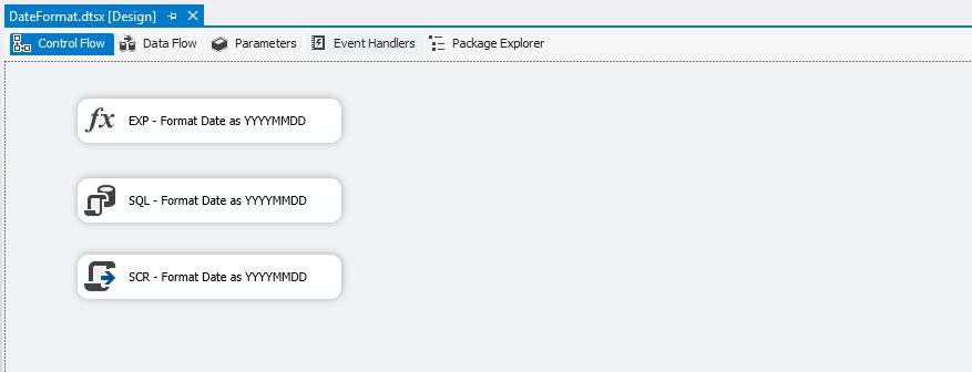
One feature that I would like to see added to SSIS is the ability to format a date string with a specified format. I have been tasked many times with outputting file names or folders with a specific date format, such as YYYYMMDD, and found myself writing custom functionality to accomplish this task. This is not difficult in T-SQL, but in SSIS it’s not all that easy. In this blog post I am going to show a few ways that we can format a date string into a specific format. I will show how to use an Expression task, SQL task, and a Script task.

Expression Task

EXP – Format Date as YYYMMDD
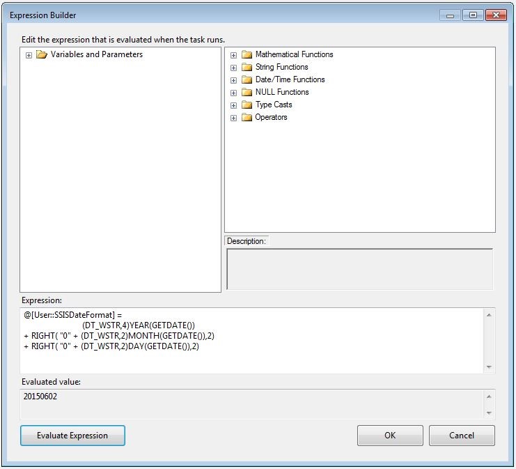
The expression task is a new features with 2012 which allows us to store the result of an expression in a variable. Basically we create an expression using the Expression Builder window and store the result into a SSIS variable. In the windows below you can see an example of the expression being set to the SSISDateFormat variable.

@[User::SSISDateFormat] =  
               (DT_WSTR,4)YEAR(GETDATE())  
+ RIGHT ( "0" + (DT_WSTR,2)MONTH(GETDATE()),2) 
+ RIGHT ( "0" + (DT_WSTR,2)DAY(GETDATE()),2)

SQL Task

SQL – Format Date as YYYYMMDD
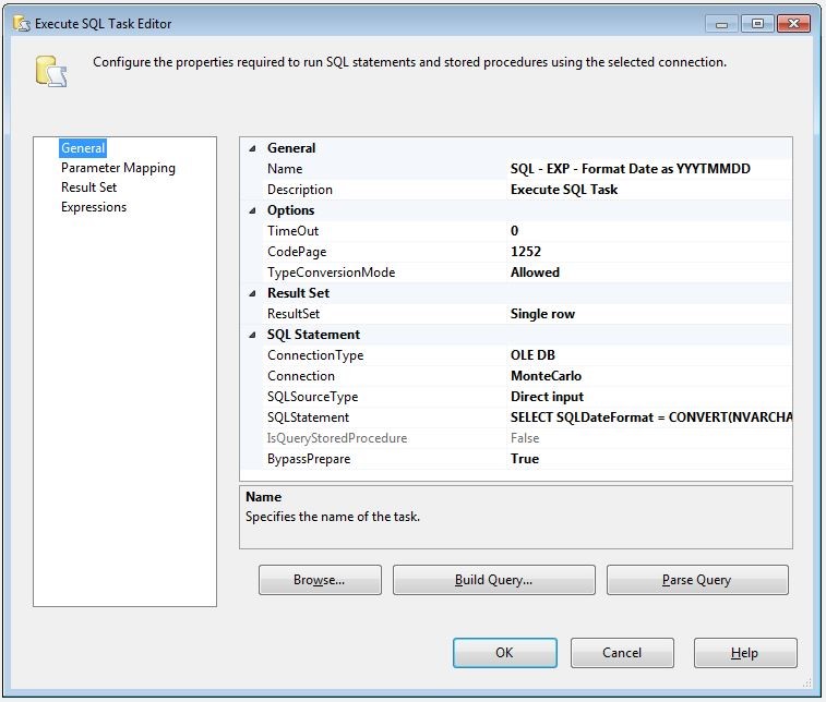
The SQL Task is a commonly used task in SSIS. This task allows us to execute queries against a data source and return a full result set, a single row, or nothing at all. We also have the opportunity to pass variables into the query as well. However, for this example we will not pass anything in, and only return back a single row. Using T-SQL’s CONVERT function it’s very easy to format a date string. We will use this CONVERT function and return the single row and store the results into a SSIS Variable. The SQL syntax that we will use is:

SELECT SQLDateFormat = CONVERT(NVARCHAR(8),GETDATE(),112);

Here is a link to additional formats for the CONVERT function. https://technet.microsoft.com/en-us/library/ms187928.aspx

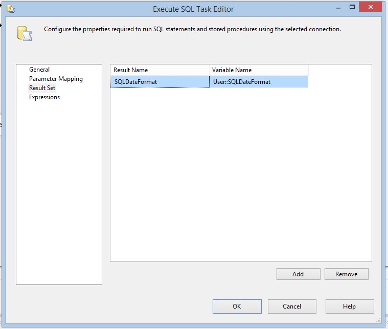
After the SQL Task executes the result will be stored in the SQLDateFormat SSIS variable, which is configured in the window below.

Script Task

SCR – Format Date YYYYMMDD
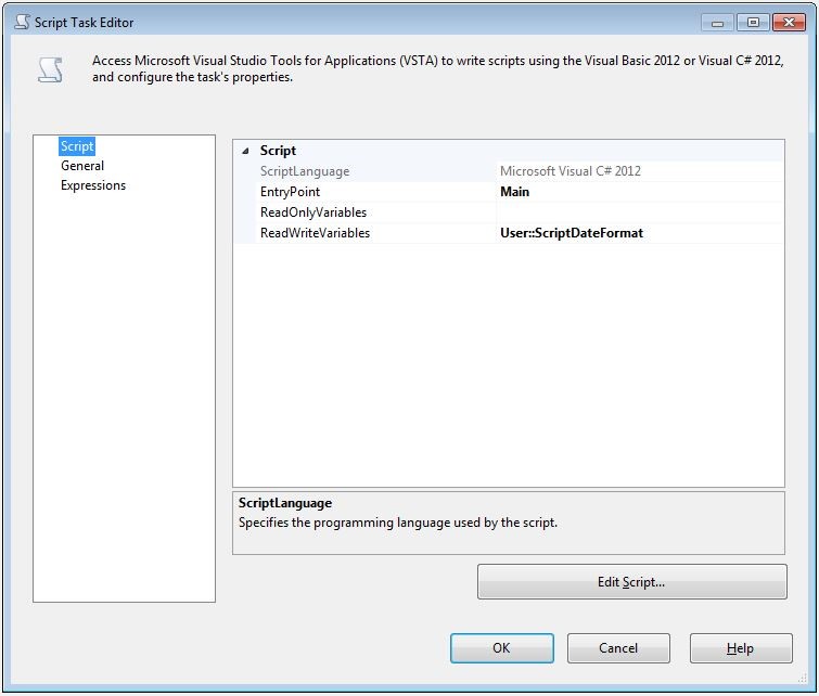
The script task is one of my favorite tasks, mainly because all of the additional functionality that I have access too, but it also gives me an opportunity to play with C#.net code. By passing the SSIS variable ScriptDateFormat into the ReadWriteVariables box, we can access that variable through code. In programming languages like C#.net it’s very easy to format a date string. There is a ToString() method that provides many date formats by using specific characters. When we click on the Edit Script button the Visual Studio for Apps design time environment appears. We can access the ScriptDateFormat variable through the Dts.Variables array and save string values to it. The result of C#.net DateTime.Now.ToString(“yyyyMMdd”) method call will give us a formatted date, this formatted date we can save to our Dts.Variables array. To get a date in T-SQL we use the GETDATE and in C#.net we use DateTime.Now. So the entire line of code would look like this.

Dts.Variables["ScriptDateFormat"].Value = DateTime.Now.ToString("yyyyMMdd");

Here is a link to MSDN page that has the format specifiers.
https://msdn.microsoft.com/en-us/library/8kb3ddd4.aspx

Summary

So which is the best way? I personally prefer the Script task, mainly because it’s clean and simple. The Expression Task is a complicated expression, and the SQL Task involves an unnecessary round trip to the server to get a formatted date string. With that said, all three options work and I am sure there are other ways as well.

LAG() and LEAD() Analytical Window Functions

I have been finding more and more uses for the OVER statement recently and I figured it was about time I did a blog post on it. The OVER statement captures a window of data that can be aggregated and included with the details of the original result set. There are a set of window functions that can be applied to the OVER statement to generate row numbers, ranking values, averaging, getting previous values and next values in a set. This idea of getting the previous and next values, in a set of data, is a problem that I just ran into recently. This blog post will describe the usage of LAG and LEAD analytical functions. LAG and LEAD are two new Analytical Window Functions that were introduced in SQL Server 2012.

Recently I was tasked with calculating the difference between two values, however the values existed in different rows. My first thought was a self-join on the table and compare the two results. Using Adventure Works 2012, I ran the following query and the results are shown.

SELECT   soh.PurchaseOrderNumber
       , soh.OrderDate
       , soh.CustomerID
       , PreviousTotal = soh1.TotalDue
       , CurrentTotal = soh.TotalDue
       , NextTotal = soh2.TotalDue
FROM     Sales.SalesOrderHeader soh
JOIN     Sales.SalesOrderHeader soh1 ON soh1.SalesOrderID = soh.SalesOrderID - 1
JOIN     Sales.SalesOrderHeader soh2 ON soh2.SalesOrderID = soh.SalesOrderID + 1;

This result set shows the previous and next record values for the TotalDue column. This got me 1/2 way to what was needed to perform the difference calculations. I needed the results for a given customer rather than all customers. I updated the query to allow for a customer ID to be passed into the query and the results are shown.

DECLARE @CustomerID int = 30117;
SELECT   soh.PurchaseOrderNumber
       , soh.OrderDate
       , soh.CustomerID
       , PreviousTotal = soh1.TotalDue
       , CurrentTotal = soh.TotalDue
       , NextTotal = soh2.TotalDue
FROM     Sales.SalesOrderHeader soh
LEFT JOIN Sales.SalesOrderHeader soh1 ON soh1.SalesOrderID = soh.SalesOrderID - 1
                                         AND soh1.CustomerID = soh.CustomerID
LEFT JOIN Sales.SalesOrderHeader soh2 ON soh2.SalesOrderID = soh.SalesOrderID + 1
                                         AND soh2.CustomerID = soh.CustomerID
WHERE    soh.CustomerID = @CustomerID;

This is was a problem. Being that I was using the SalesOrderID to perform the self-joins on the tables, and the Customer’s records were not in sequential order, I was not getting any of the previous and next records.

LEAD()/LAG() OVER (PARTITION BY)

Instead of going down the path of craziness, I decided to eliminate the use of the self-referencing joins and opted to use the OVER clause with LEAD and LAG to solve the problem. Using the following query and output we can explain the LEAD(), LAG(), OVER (PARTITION BY) statements.

DECLARE @CustomerID int = 30117;
SELECT   PurchaseOrderNumber
       , OrderDate
       , CustomerID
       , CurrentTotalDue = TotalDue
FROM     Sales.SalesOrderHeader soh
WHERE    soh.CustomerID = @CustomerID;

In the blue box is the CustomerID column, this is the column we want to Partition by.

In the red box is the PurchaseOrderNumber and OrderDate columns, these columns we want to order the results of the window.

In the green box is the CurrentTotalDue, this is the column that we will pass to the LEAD and LAG window functions.

I updated the query to use the LEAD and LAG window functions and the results are shown. The red highlights show the results of the LEAD function and the green highlights show the results of the LAG function.

DECLARE @CustomerID int = 30117;
SELECT   PurchaseOrderNumber
       , OrderDate
       , PreviousTotal = LAG(TotalDue) OVER (PARTITION BY CustomerID ORDER BY OrderDate , PurchaseOrderNumber)
       , CurrentTotal = TotalDue
       , NextTotal = LEAD(TotalDue) OVER (PARTITION BY CustomerID ORDER BY OrderDate , PurchaseOrderNumber)
FROM     Sales.SalesOrderHeader soh
WHERE    soh.CustomerID = @CustomerID;

As you can see the syntax for writing a query to use these LEAD and LAG are not overly complex. In a future blog post I will dive deeper into using the OVER statement.

Standard T-SQL UNPIVOT

In prior blog posts I talked about a Standard PIVOT query and a Dynamic PIVOT query. It is only fitting that I talk about how to implement an UNPIVOT query. As DBA’s we commonly unpivot data and turn it into normalized data for storing in a relational data store. Understanding how to use the UNPIVOT query is a great skill to have as a DBA. Just like the PIVOT operator, the UNPIVOT operator was introduced with SQL Server 2005. In this blog post I will show how we can use the UNPIVOT operator.

I got the idea for this blog post as a result from my online grade book. I noticed that the data is displayed as a denormalized set of data. As an instructor I thought it would be interesting to see average, sum, minimum and maximum assignment scores for each student. Below is an example of the display of the online grade book.

StudentID	Assignment1	Assignment2	Assignment3	Assignment4
101	90	100	95	100
102	70	65	40	80
103	100	100	100	100

I found that writing a simple query to get the sum (adding each column) and average (adding each column and dividing by the number of columns) was not too bad. However, finding the minimum and maximum proved to be a bit tricky. Sure we could implement a CASE WHEN statement, however for each column the complexity and possibility of error increases significantly, and maintainability dang near goes out the window. In comes UNPIVOT to save the day. After unpivoting the data, we simply use the AVG(), SUM(), MIN() and MAX() functions.

Let’s take a look at the basic structure of the UNPIVOT query. Using the UNPIVOT statement, you specify a value and data column, then select each of the columns you want to unpivot into these new columns. The new value and data columns become select-able columns in the query, as shown in the following code.

SELECT   [AnyColumn]
       , [DataColumn]
       , [ValueColumn]
FROM     SomeTable ST 
UNPIVOT ( ValueColumn FOR DataColumn IN (UnPivotCol1, UnPivotCol2, UnPivotCol2) ) AS UNPVT

Applying this UNPIVOT syntax to our data above we yield the following query.

SELECT   StudentID
       , Assignment
       , ASMT.Score
FROM     #ClassGrades CG 
UNPIVOT ( Score FOR Assignment IN (Assignment1, Assignment2, Assignment3, Assignment4) ) AS ASMT

This query returns the following normalized view of the data

StudentID	Assignment	Score
101	Assignment1	90
101	Assignment2	100
101	Assignment3	95
101	Assignment4	100
102	Assignment1	70
102	Assignment2	65
102	Assignment3	40
102	Assignment4	80
103	Assignment1	100
103	Assignment2	100
103	Assignment3	100
103	Assignment4	100

Now that we have this data in a normalized result, applying SQL functions such as AVG() and SUM(), is relatively simple. Below is an updated version of the query using the AVG(), SUM(), MIN(), and MAX() functions grouping by StudentID.

SELECT   StudentID
       , Average = AVG(ASMT.Score)
	   , MaxScore = MAX(ASMT.Score)
	   , MinScore = MIN(ASMT.Score)
	   , Total = SUM(ASMT.Score)
FROM     #ClassGrades CG 
UNPIVOT ( Score FOR Assignment IN (Assignment1, Assignment2, Assignment3, Assignment4) ) AS ASMT
GROUP BY StudentID

This query returns the following view of the data

StudentID	Average	MaxScore	MinScore	Total
101	96	100	90	385
102	63	80	40	255
103	100	100	100	400

As you can see the PIVOT and UNPIVOT statements are not overly complex and are definitely great TSQL tools for any DBA to keep in their back-pocket. Below is the entire script with test data included.

IF OBJECT_ID('tempdb..#ClassGrades') IS NOT NULL 
   DROP TABLE #ClassGrades;
 
CREATE TABLE #ClassGrades (
   StudentID int PRIMARY KEY
                 NOT NULL
 , Assignment1 int NULL
 , Assignment2 int NULL
 , Assignment3 int NULL
 , Assignment4 int NULL);
 
INSERT   INTO #ClassGrades
         (StudentID, Assignment1, Assignment2, Assignment3, Assignment4)
VALUES   (101, 90, 100, 95, 100),
         (102, 70, 65, 40, 80),
         (103, 100, 100, 100, 100); 
 
SELECT   StudentID
       , Assignment
       , ASMT.Score
FROM     #ClassGrades CG 
UNPIVOT ( Score FOR Assignment IN (Assignment1, Assignment2, Assignment3, Assignment4) ) AS ASMT
 
SELECT   StudentID
       , Average = AVG(ASMT.Score)
	   , MaxScore = MAX(ASMT.Score)
	   , MinScore = MIN(ASMT.Score)
	   , Total = SUM(ASMT.Score)
FROM     #ClassGrades CG 
UNPIVOT ( Score FOR Assignment IN (Assignment1, Assignment2, Assignment3, Assignment4) ) AS ASMT
GROUP BY StudentID;

Rules of Engagement – NoSQL Graph Databases

Well Rick Krueger( blog | @DataOgre ) and I are back at it again. We have decided to pair up and do a talk about a rather controversial topic in the SQL Server community, NoSQL. Now we are not jumping ship and saying that NoSQL is the way of the future, because that is simply not true. Relational databases have been around since the 70′s and still outperform NoSQL Solutions at most tasks. The idea that we are going to seed is that these NoSQL solutions may have a place in enterprise applications. We are not going to say you should use SQL Server or a NoSQL Solution exclusively, rather we are going to claim Polyglot Persistence. Polyglot Persistence is the idea of using multiple data stores to solve multiple problems, hence Rules of Engagement: NoSQL is SQL Server’s Ally. In a previous blog post I discussed Key Value Stores and Column Stores, in this blog post I will be discussing another version of the NoSQL solutions, Graph Databases.

Graph Databases

Graph Databases are data structures that consist of nodes, properties, and edges. In RDBMS terms a node would be a record in a table, a property would be the data within the record, and an edge would be similar to the relationship between tables. However the edges can store properties too, these properties describe the relationship between the nodes.

In the RDBMS land, writing queries to join many large tables, especially self referencing tables, can degrade performance of a query and can be rather costly, even with proper index usage. This is where Graph databases really shine, the graph databases has the ability traverse nodes using the edges and the properties within the edges. Using Graph Database to find relationships between highly interconnected data is very fast. Finding data that would take multiple joins or a recursive query in a RDBMS is a simple task with Graph Databases.

You can visualize a graph database as a flattened RDBMS table structure with named connections. Looking at the the relational tables below we see simple car buying and selling database. This database has a list of cars that people currently own and the types of cars they are looking for. If we were to flatten and denormalize the structure we would get something that looks like this.

Here the Car node is the CarType and Manufacture tables denormalized, the Person node is the Person table, and the edges that connect these two nodes would be the Request and Cars tables. Depending on the data you are looking for, both of these structures have their merits. Lets say you need to write a query that will return a list cars for a given owner that is willing to trade with another owner. This is a simple query for both, however what if there is not a match, but there is a match using a 3rd party for a trade. Or maybe there needs to be a 4th or 5th party for a four or five way trade. This query is starting to get very complicated in a RDBMS, and the performance at each level is progressively degrading. This is where a Graph Database is really going to stand out! Being that the emphasis is on the edges between the nodes, the query is simple and will give you performance your application will desire.

Graph Database Implementations

One of the most recognized Graph Databases implementations is Neo4j and is currently made available by Neo Technologies.

“Neo4j is a robust (fully ACID) transactional property graph database. Due to its graph data model, Neo4j is highly agile and blazing fast. For connected data operations, Neo4j runs a thousand times faster than relational databases.” – http://www.neo4j.org/

Neo4j is available for most platforms and comes with a WebAdmin management console for viewing the graph database. Below are some screen captures of the Web Admin utility showing a Dashboard for over all database health, and some ways to view the data inside the database.

Polyglot Persistence, SQL Server and Graph Databases

Recently Facebook announced a graph search feature in their application.

“With graph search you can look up anything shared with you on Facebook, and others can find stuff you’ve shared with them.” – https://www.facebook.com/about/graphsearch

This is idea of using a graph database within their application is the idea behind polyglot persistence. Their primary data could be stored in any data structure such as a RDBMS, but their graph search feature would be stored in a Graph Database.

Conclusion

I am not recommending that you re-write your applications to make room for a NoSQL solution, I am simply suggesting that you as the DBA (keeper of data), should keep an open mind to other possibilities. If there is another solution out there that could assist SQL Server, or is maybe a better fit, exploring the avenue might result in a better data solution. As always, a round peg will fit into a square hole if you have a big enough hammer.

Rules of Engagement – Key Value Stores

Well Rick Krueger( blog | @DataOgre ) and I are back at it again. We have decided to pair up and do a talk about a rather controversial topic in the SQL Server community, NoSQL. Now we are not jumping ship and saying that NoSQL is the way of the future, because that is simply not true. Relational databases have been around since the 70’s and still outperform NoSQL Solutions at most tasks. The idea that we are going to seed is that these NoSQL solutions may have a place in enterprise applications. We are not going to say you should use SQL Server or a NoSQL Solution exclusively, rather we are going to claim Polyglot Persistence. Polyglot Persistence is the idea of using multiple data stores to solve multiple problems, hence Rules of Engagement: NoSQL is SQL Server’s Ally. In this blog post I will be discussing the simplest version of the NoSQL solutions, Key Value Stores.

Key Value Stores

There are many Key Value store implementations, however at the root of each solution, they are simply storing values by a specific key. You can think of this as a two column table, a hash table, or an associative array.
They use a unique indexed key, which allows for fast retrieval of data, and a blob type of field for the value. The key value stores are typically written in some type of programming language, commonly Java. This gives the application developer the freedom to store data how they see fit, in a schema-less data store. Yes I used application developer, freedom, data, and schema-less all in the same sentence. This is a good thing. Typically we, as the DBA’s, are not going to be distracted by how the data is stored in the Key Value Store. Rather, we will be involved with serving up the data that will be pushed into the Key Value store, and helping with any transaction support that is needed.

One of the biggest benefit for most NoSQL solutions, including Key Value Stores, would be horizontal scaling. We all know that horizontal scaling and SQL Server, while it’s possible, does not play well. Typically if you need more from SQL Server you scale vertically, which can be costly.

Another benefit for Key Value stores is a lack of schema, this allows for changing the data structure as needed, thus being a bit more flexible. Whereas with SQL Server altering a table could result in stored procedures, functions, views, etc… needing updates, which take time and a DBA resource.

Key Value stores support “Eventual Consistency”, if a feature in your application doesn’t need to fully support ACID, then may not be a significant draw back. However the features of your application that need ACID transaction support should use a RDBMS, like SQL Server.

Another drawback is querying data from a Key Value store. Simple queries for keys in Key Value stores are a minor task because they are indexed. However, supporting joins or complex queries takes coding by an application developer. Code developed queries lose out on years of SQL Server optimization and caching features.

A Key Value Store Implementation

Redis
Redis is an advanced Key Value store, meaning that it can support more complex data types such as Lists, Objects, Hashes, Sets, etc… Redis is a combination of an in-memory and persisted to disk data store. This gives Redis great performance on reads and writes, however it puts a limitation on what can be stored, as memory becomes a constraint. The basic commands for CRUD operations in Redis are rather simple: GET, SET, and DEL. http://try.redis.io/ offers an online utility for learning some of the commands.

Polyglot Persistence, SQL Server and Key Value Stores

Obviously there are pros and cons for Key Value Stores, however creating a hybrid solution, could solve the drawbacks for both SQL Server and Key Value Stores. Every application is different and ultimately you will need to decide what the best fit is, for your application and budget.

With that said an example for a Key Value Store could be session data. Where the session id would be the key and all the session data would be in the value. An in-memory database, such as Redis, could produce quick results to the UI, significantly improving the web applications performance. However when that session ends, all of the updated detailed user information would ultimately need to be persisted, let’s say in a SQL Server Users table.

Or maybe a shopping cart feature, again the shopping cart id would be the key and the contents of the shopping cart would be in the value. What happens when the user checks out? That’s right, we will need to store that transaction, user information, product information, and inventory into a RDBMS such as SQL Server

Conclusion

I am not recommending that you re-write your applications to make room for a NoSQL solution, I am simply suggesting that you as the DBA (keeper of data), should keep an open mind to other possibilities. If there is another solution out there that could assist SQL Server, or is maybe a better fit, exploring the avenue might result in a better data solution. A square object will fit into a round hole if you have a big enough hammer, but could take time and produce a bad product.

Dave + SQL Server = Ingenious SQL….

SQL Thoughts from @IngeniousSQL

Category: SQL

Simple SSIS: Date Formats

LAG() and LEAD() Analytical Window Functions

Standard T-SQL UNPIVOT

Rules of Engagement – NoSQL Graph Databases

Rules of Engagement – Key Value Stores