Dave + SQL Server = Ingenious SQL....

Simple SSIS: Traversing Files in a Directory

There are many common daily tasks that (SSIS) SQL Server Integration Services implements with minimal effort. These tasks can be done by adding a few SSIS tasks, data flows, and containers. In this blog series I am going to explore some of these simple tasks and how I go about implementing them. Looping through a directory of files definitely qualifies as simple task using SSIS. In this blog post I will show how to traverse a set of files and log the files found using SSIS. This blog post builds on a previous Simple SSIS blog post, Importing Data from Flat Text Files

Prerequisites

We will need a database table called FileImport, which will store the file details, for the File Loop SSIS package.

FileImport

The File Import table is the historical logging table. This table contains all of the file details, such as start and end time, if it was imported of if an error occurred, as well as a path to the file.

CREATE TABLE dbo.FileImport (
     FileImportID INT IDENTITY(1, 1) NOT NULL
   , FileName NVARCHAR(1000) NOT NULL
   , ImportStartDate DATETIME NULL
   , ImportEndDate DATETIME NULL
   , RecordCount INT NULL
   , Imported BIT NULL
   , ErrorMessage NVARCHAR(MAX) NULL
   , CONSTRAINT PK_FileImport PRIMARY KEY CLUSTERED (FileImportID ASC)
) ON  [PRIMARY];

File Loop SSIS package

The File Loop SSIS package will traverse a specified folder capturing the path of each file stored in the folder. For each file, we will write some basic file details to a log table and import data from the file into a file details table. The details of the file import is left to a previous Simple SSIS blog post.

Let’s start by creating a new SSIS Package and renaming it to FileLoop.dtsx. The package will need a couple variables which are defined below.

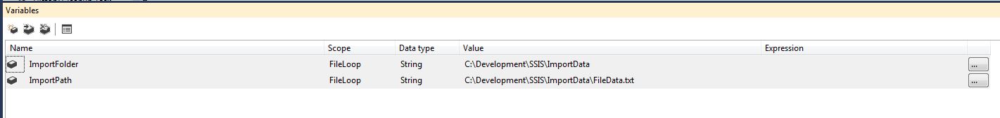
Variable Definitions

The ImportFolder is the folder where all of the files to be imported are stored.
The ImportPath is the actual path to each file. This will be updated on each iteration of the foreach loop container.

Package Tasks

The File Loop package will use a Foreach Loop Container, an Execute SQL Task, and a Data Flow Task.

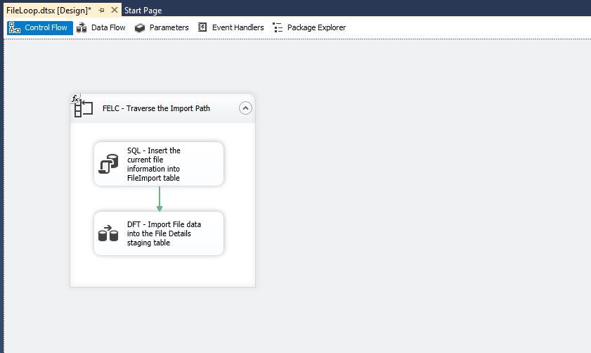
FELC – Traverse the Import Path

This Foreach Loop Container will traverse the list of files that are stored in the designated folder. Using an expression we can dynamically set the Directory/Folder at runtime. For this import we are only looking for files that start with FileData and have a .txt extension. We will want the fully qualified path to the file and do not want to traverse the sub folders.

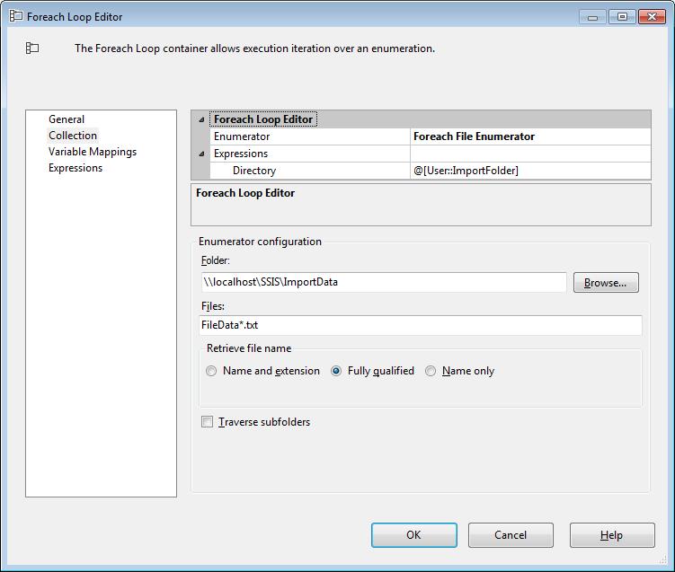
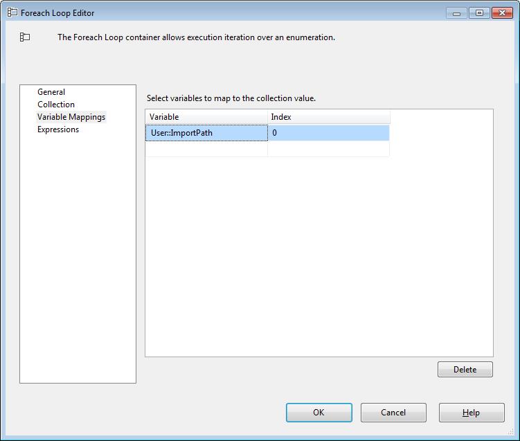
On each iteration of the loop we will save the path to each of the files in the ImportPath SSIS variable.

SQL – Insert the current file information into FileImport table

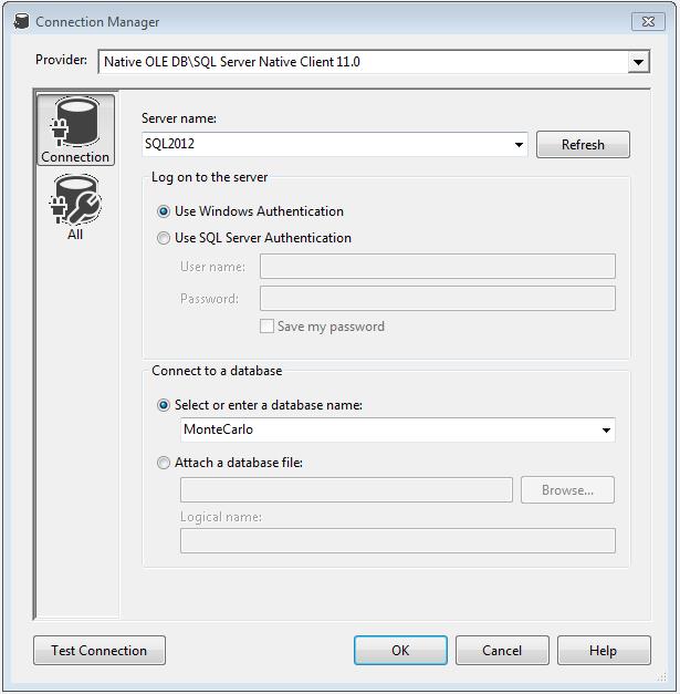
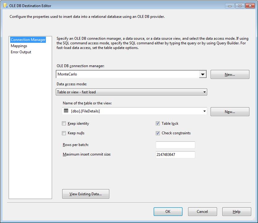
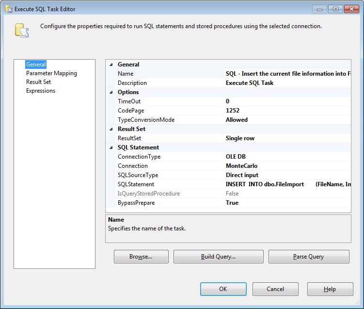
This Execute SQL Task will create a new entry into the FileImport Table and return the newly inserted identity value. We will need to set the Result Set to Single Row to capture the identity returned from the INSERT statement. Select the Connection type of OLE DB and the previously setup Connection. We will use a simple SQL Statement to Insert The file name and start date and return the identity.

INSERT  INTO dbo.FileImport (FileName, ImportStartDate)
VALUES  (?, GETDATE());
SELECT FileImportID = @@IDENTITY;

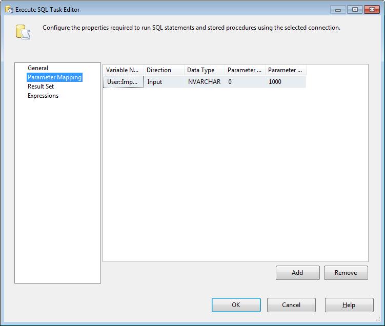
We are only using a single input parameter so we will need to add and map the ImportPath variable. Select the Data Type as NVARCHAR, Parameter Name = 0, and Parameter Size = 1000.
NOTE: The Parameter Names are a numerical ordering because we are using OLE DB Connections. For other types of connection types see Parameters and Return Codes in the Execute SQL Task, https://msdn.microsoft.com/en-us/library/cc280502.aspx

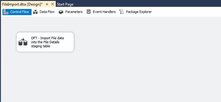
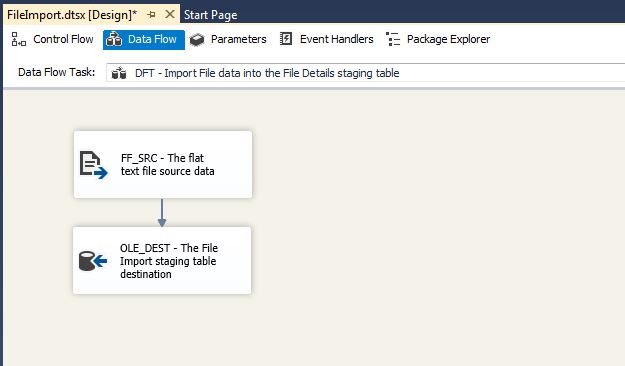
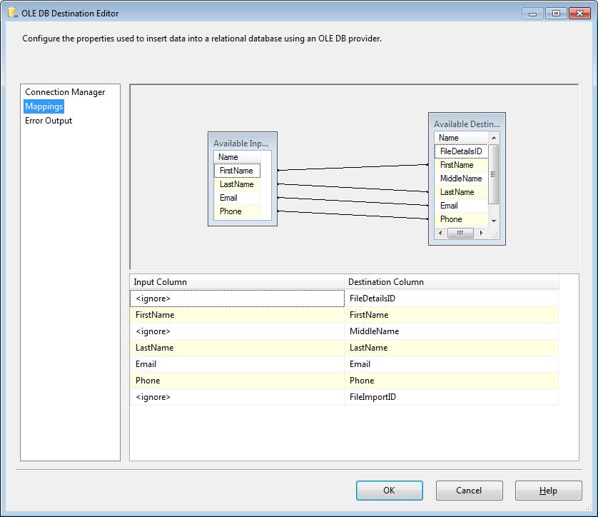
DFT – Import File data into the File Details staging table

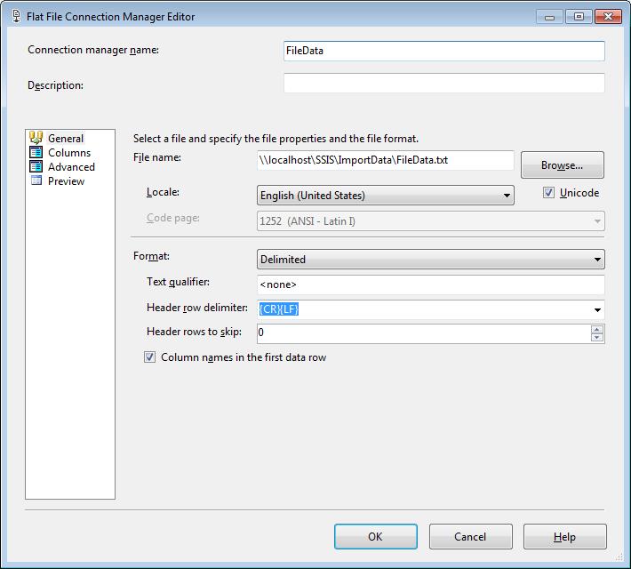
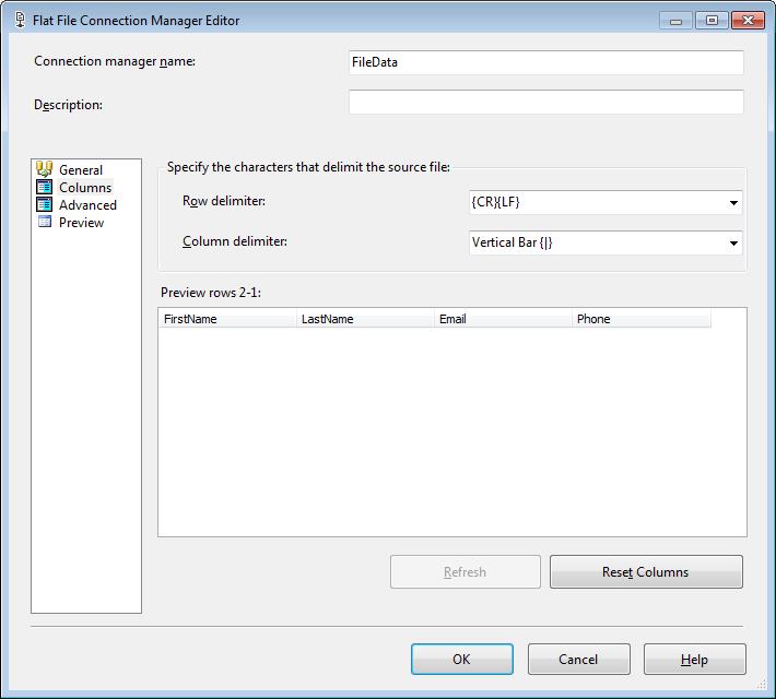
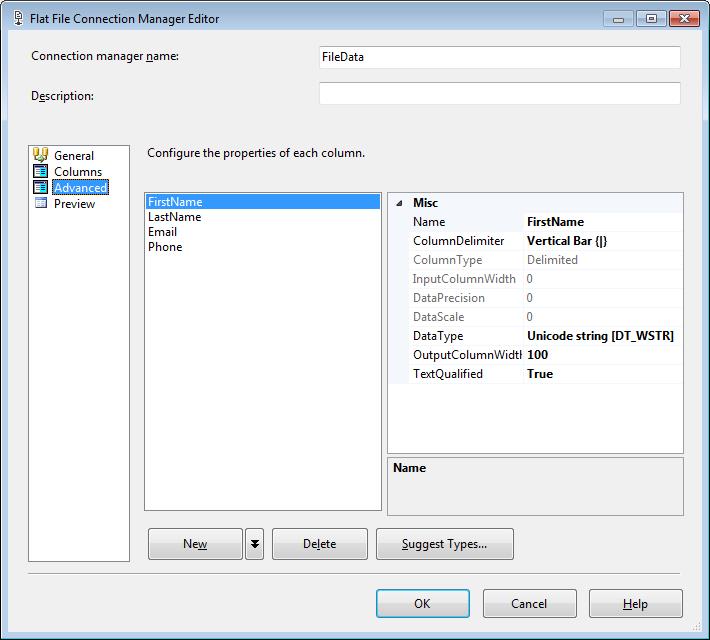
This Data Flow Task will be used to import each of the files into a staging table. In another Simple SSIS blog post the details for the file import process is documented.

Execution

After executing the File Loop SSIS package, all of the file paths that match the pattern FileData*.txt will have been placed in a temporary SSIS string variable, which can be used for other operations such as file imports. In my next Simple SSIS blog post I will review importing data from pipe delimited flat text files.

Simple SSIS: Importing Data from Flat Text Files

There are many common daily tasks that (SSIS) SQL Server Integration Services implements with minimal effort. These tasks can be done by adding a few SSIS tasks, data flows, and containers. In this blog series I am going to explore some of these simple tasks and how I go about implementing them. Importing data from flat text files into a data store definitely qualifies as simple task using SSIS. In this blog post I will show how to import pipe-delimited files into staging tables using SSIS.

Prerequisites

A database table called FileDetails is needed, which matches the data that we are going to import from the pipe delimited flat text files.

Pipe Delimited Flat File Sample

FirstName|LastName|Email|Phone
Kieran|Merrill|dis.parturient.montes@eutellusPhasellus.org|(852) 339-2795
Dai|Figueroa|hendrerit.id.ante@adipiscingenimmi.co.uk|(553) 107-6735
Priscilla|Morrow|faucibus@Mauriseu.ca|(190) 642-4764
Raphael|Kent|nisi.Aenean.eget@hendreritaarcu.net|(262) 161-4288
Whilemina|Leblanc|Curabitur.dictum.Phasellus@quistristique.edu|(420) 952-2809
Kerry|Morrow|gravida@nonummy.org|(633) 115-7473

File Details

The File Details table is the staging table for all records imported. Each staging table will be representative of the data that is being imported. Being that the data being imported us user specific, the following columns are relevant; name, email, phone, etc…

CREATE TABLE dbo.FileDetails (
     FileDetailsID INT IDENTITY(1, 1) NOT NULL
   , FirstName NVARCHAR(100) NOT NULL
   , MiddleName NVARCHAR(100) NULL
   , LastName NVARCHAR(100) NOT NULL
   , Email NVARCHAR(100) NOT NULL
   , Phone NVARCHAR(25) NULL
   , FileImportID INT NOT NULL
   , CONSTRAINT PK_FileDetails PRIMARY KEY CLUSTERED (FileDetailsID ASC)
) ON  [PRIMARY];

File Import SSIS package

The File Import SSIS package will make a connection to a flat text file, read the contents of the flat text file into a data stream, map the results to a database connection and write the contents of the stream to a specified database table.

Let’s start by creating a new SSIS Package and renaming it to FileImport.dtsx.
We will need to setup an OLE DB connection to query the FileImport and FileDetails tables as well as a Flat File connection to read the pipe-delimited flat text file data.

OLE DB Connection

Flat File Connection

In the general section of the flat file connection manager editor we will select a file that is representative of the files that will be imported. The pipe delimited file we are going to import may contain Unicode characters and has column names in the header row, so we will need to select the “Unicode” and “Columns names in the first data row” options.

In the columns section of the flat file connection manager editor we will select the Vertical Bar {|} value for the Column delimiter drop down list, because the flat text file is pipe delimited.

In the Advanced section of the flat file connection manager editor we will need to adjust each of the columns to match the data size and type for the corresponding database column.

Package Tasks

The File Import package will use a single Data Flow task to import the file data. This Data Flow task “DFT – Import File data into the File Details staging table” implements the file import process, using a Flat File Source and OLE DB Destination.

Data Flows

DFT – Import File data into the File Details staging table

This data flow implements two components a Flat File Source and OLE DB Destination which are necessary for importing data between the flat text file and the database table.

FF_SRC – The flat text file source data

This data source will define the connection manager and the output columns from the flat text file into a data stream. This data stream will provide the input to the OLE DB Destination to write data to the files. On the connection manager section select the FileData flat file connection manager.

On the Columns section we will output all four columns. As a best practice, if you are not going to use one of the columns in the data flow, its best to deselect it hear, it will takes up less space on your data stream and increase the performance of your package.

OLE_DEST – The File Import staging table destination

This OLE DB destination will define the details of the destination of our data into the database tables and which data stream columns will be mapped to which database columns. On the connection manager section we will select our OLE DB Connection and the Data Access mode of Table of view – fast load. Select [dbo].[FileDetails] as the name of the table or view.

On the Mappings section, if the OLE DB Destination could match the names, lines will be drawn connecting the two columns. If any columns are not automatically mapped, either drag and drop the column on the corresponding columns that should be mapped, or select the corresponding column value from the Input Column dropdown list.

After the package is executed the data will be loaded into the FileDetails staging table. In a future Simple SSIS blog post I will show how to loop through a directory of files and improve on this import by capturing debugging information and import statistics.

T-SQL Bitwise Matching Logic – #TSQL2sDay

A good friend of mine Rick Kruger (@DataOgre|blog) is hosting this month’s T-SQL Tuesday Blog party. The T-SQL Tuesday Blog parties were started by Adam Machanic (@AdamMachanic|blog) back in December of 2009. This month’s topic is on Rube Goldberg Machines. Rick asked us to look through our closets to dig up a skeleton, something that we made T-SQL do, which might make other DBA’s cringe a bit. After hearing this, I knew exactly what I was going to blog about.

Bitwise Matching!

I remember when I implemented this feature and shook my head when I came up with the idea of using bitwise matching. The requirements I was given was to match two entities based on assigned lookup values. This would not have been that bad, except the lookup values were not static, they were dynamically entered through a web UI. When I first pitched the idea I used a dating site as a way to explain the logic, so in this blog post I will use that same concept.

Concept

Within a dating site one person is matched to another based on activities they both enjoy. Activities can be grouped into different categories. In this example we have two different categories; Exercise and Things to do. People must have at least one matching activity in each category to be a match. We are going to try to match Bob with another person.

People and their activities

Bob enjoys Walking, Biking, and Camping.
Sally enjoys Walking and Biking
Nancy enjoys Camping
Beth enjoys Walking, Running, Golfing, and Camping.

The following T-SQL implements a few temporary tables we will use to implement the bitwise matching logic.

-- Create the People that can be matched.
CREATE TABLE #Person (
   PersonID smallint
 , Name nvarchar(25));
INSERT   INTO #Person
         (Name)
VALUES   (1, N'Bob'), (2, N'Sally'), (3, N'Nancy'), (4, N'Beth');
 
-- Create the Activities that people may have in common.
CREATE TABLE #Activities (
   ActivityID smallint
 , Activity nvarchar(25)
 , CategoryID smallint);
 
INSERT   INTO #Activities
         (Activity, CategoryID)
VALUES   (1, N'Walking', 1), (2, N'Biking', 1), (3, N'Running', 1), (4, N'Yoga', 1),        
	 (5, N'Movies', 2), (6, N'Golf', 2), (7, N'Camping', 2);
 
-- Create the Weak Entity Table to store the Persons Activities.
CREATE TABLE #PersonActivities (
   ActivityID smallint
 , PersonID smallint);
 
INSERT   INTO #PersonActivities
         (PersonID, ActivityID)
VALUES   (1, 1), (1, 2), (1, 7),
         (2, 1),(2, 2),
         (3, 7),
         (4, 1),(4, 3),(4, 6),(4, 7);

Bitwise Logic

Using the activities we can assign a bitwise value based on the identity and category.
Example:

Activity	Activity ID	Category ID	Bitwise Value
Walking	1	1	2¹ = 2
Biking	2	1	2² = 4
Running	3	1	2³ = 8
Yoga	4	1	2⁴ = 16
Movies	1	2	2¹ = 2
Golf	2	2	2² = 4
Camping	3	2	2³ = 8

If we summarize the bitwise values we can use the binary and operator (&) to determine if any matches exist. Example:

Summed Bitwise Value		2³	2²	2¹	2⁰
6	=	0	1	1	0
12	=	1	1	0	0

4	=	0	1	0	0

The value of 6 represents Walking and Biking, the value of 12 represents Biking and Running. The intersection of the two is Biking, this would be the matched value of 4. Being that we have a matched value, the result is greater than 0. Using this logic we can implement the following query.

WITH  PeopleSums
        AS (
            SELECT   p.Name
                   , p.PersonID
                   , a.CategoryID
                   , BitWiseSum = SUM(POWER(2, pa.ActivityID))
            FROM     #Person p
            JOIN     #PersonActivities pa ON p.PersonID = pa.PersonID
            JOIN     #Activities a ON a.ActivityID = pa.ActivityID
            GROUP BY p.Name
                   , p.PersonID
                   , a.CategoryID
           )
   SELECT   ps2.Name
   FROM     PeopleSums ps
   JOIN     PeopleSums ps2 ON ps.PersonID != ps2.PersonID
                              AND ps.BitWiseSum & ps2.BitWiseSum <> 0
                              AND ps.CategoryID = ps2.CategoryID
   WHERE    ps.Name = 'Bob'
   GROUP BY ps.Name
          , ps2.Name
   HAVING   COUNT(*) = 2;

This query uses a CTE to calculate and then summarize the bitwise values, grouped by person and category. We then self-reference the CTE using the binary AND operator (&) where the result is anything but zero. This concept can show us who Bob matches, we can use the table below to illustrate this.

Persons that Match Bob	Category 1	Category 2
Sally	Walking, Biking
Nancy		Camping
Sally	Walking	Camping

To make sure that we have a match for each category, we do a count and ensure that it matches the number of categories we currently have. And voila Beth is a match for Bob, because Beth is the only candidate that had matches in both categories.

LAG() and LEAD() Analytical Window Functions

I have been finding more and more uses for the OVER statement recently and I figured it was about time I did a blog post on it. The OVER statement captures a window of data that can be aggregated and included with the details of the original result set. There are a set of window functions that can be applied to the OVER statement to generate row numbers, ranking values, averaging, getting previous values and next values in a set. This idea of getting the previous and next values, in a set of data, is a problem that I just ran into recently. This blog post will describe the usage of LAG and LEAD analytical functions. LAG and LEAD are two new Analytical Window Functions that were introduced in SQL Server 2012.

Recently I was tasked with calculating the difference between two values, however the values existed in different rows. My first thought was a self-join on the table and compare the two results. Using Adventure Works 2012, I ran the following query and the results are shown.

SELECT   soh.PurchaseOrderNumber
       , soh.OrderDate
       , soh.CustomerID
       , PreviousTotal = soh1.TotalDue
       , CurrentTotal = soh.TotalDue
       , NextTotal = soh2.TotalDue
FROM     Sales.SalesOrderHeader soh
JOIN     Sales.SalesOrderHeader soh1 ON soh1.SalesOrderID = soh.SalesOrderID - 1
JOIN     Sales.SalesOrderHeader soh2 ON soh2.SalesOrderID = soh.SalesOrderID + 1;

This result set shows the previous and next record values for the TotalDue column. This got me 1/2 way to what was needed to perform the difference calculations. I needed the results for a given customer rather than all customers. I updated the query to allow for a customer ID to be passed into the query and the results are shown.

DECLARE @CustomerID int = 30117;
SELECT   soh.PurchaseOrderNumber
       , soh.OrderDate
       , soh.CustomerID
       , PreviousTotal = soh1.TotalDue
       , CurrentTotal = soh.TotalDue
       , NextTotal = soh2.TotalDue
FROM     Sales.SalesOrderHeader soh
LEFT JOIN Sales.SalesOrderHeader soh1 ON soh1.SalesOrderID = soh.SalesOrderID - 1
                                         AND soh1.CustomerID = soh.CustomerID
LEFT JOIN Sales.SalesOrderHeader soh2 ON soh2.SalesOrderID = soh.SalesOrderID + 1
                                         AND soh2.CustomerID = soh.CustomerID
WHERE    soh.CustomerID = @CustomerID;

This is was a problem. Being that I was using the SalesOrderID to perform the self-joins on the tables, and the Customer’s records were not in sequential order, I was not getting any of the previous and next records.

LEAD()/LAG() OVER (PARTITION BY)

Instead of going down the path of craziness, I decided to eliminate the use of the self-referencing joins and opted to use the OVER clause with LEAD and LAG to solve the problem. Using the following query and output we can explain the LEAD(), LAG(), OVER (PARTITION BY) statements.

DECLARE @CustomerID int = 30117;
SELECT   PurchaseOrderNumber
       , OrderDate
       , CustomerID
       , CurrentTotalDue = TotalDue
FROM     Sales.SalesOrderHeader soh
WHERE    soh.CustomerID = @CustomerID;

In the blue box is the CustomerID column, this is the column we want to Partition by.

In the red box is the PurchaseOrderNumber and OrderDate columns, these columns we want to order the results of the window.

In the green box is the CurrentTotalDue, this is the column that we will pass to the LEAD and LAG window functions.

I updated the query to use the LEAD and LAG window functions and the results are shown. The red highlights show the results of the LEAD function and the green highlights show the results of the LAG function.

DECLARE @CustomerID int = 30117;
SELECT   PurchaseOrderNumber
       , OrderDate
       , PreviousTotal = LAG(TotalDue) OVER (PARTITION BY CustomerID ORDER BY OrderDate , PurchaseOrderNumber)
       , CurrentTotal = TotalDue
       , NextTotal = LEAD(TotalDue) OVER (PARTITION BY CustomerID ORDER BY OrderDate , PurchaseOrderNumber)
FROM     Sales.SalesOrderHeader soh
WHERE    soh.CustomerID = @CustomerID;

As you can see the syntax for writing a query to use these LEAD and LAG are not overly complex. In a future blog post I will dive deeper into using the OVER statement.

Standard T-SQL UNPIVOT

In prior blog posts I talked about a Standard PIVOT query and a Dynamic PIVOT query. It is only fitting that I talk about how to implement an UNPIVOT query. As DBA’s we commonly unpivot data and turn it into normalized data for storing in a relational data store. Understanding how to use the UNPIVOT query is a great skill to have as a DBA. Just like the PIVOT operator, the UNPIVOT operator was introduced with SQL Server 2005. In this blog post I will show how we can use the UNPIVOT operator.

I got the idea for this blog post as a result from my online grade book. I noticed that the data is displayed as a denormalized set of data. As an instructor I thought it would be interesting to see average, sum, minimum and maximum assignment scores for each student. Below is an example of the display of the online grade book.

StudentID	Assignment1	Assignment2	Assignment3	Assignment4
101	90	100	95	100
102	70	65	40	80
103	100	100	100	100

I found that writing a simple query to get the sum (adding each column) and average (adding each column and dividing by the number of columns) was not too bad. However, finding the minimum and maximum proved to be a bit tricky. Sure we could implement a CASE WHEN statement, however for each column the complexity and possibility of error increases significantly, and maintainability dang near goes out the window. In comes UNPIVOT to save the day. After unpivoting the data, we simply use the AVG(), SUM(), MIN() and MAX() functions.

Let’s take a look at the basic structure of the UNPIVOT query. Using the UNPIVOT statement, you specify a value and data column, then select each of the columns you want to unpivot into these new columns. The new value and data columns become select-able columns in the query, as shown in the following code.

SELECT   [AnyColumn]
       , [DataColumn]
       , [ValueColumn]
FROM     SomeTable ST 
UNPIVOT ( ValueColumn FOR DataColumn IN (UnPivotCol1, UnPivotCol2, UnPivotCol2) ) AS UNPVT

Applying this UNPIVOT syntax to our data above we yield the following query.

SELECT   StudentID
       , Assignment
       , ASMT.Score
FROM     #ClassGrades CG 
UNPIVOT ( Score FOR Assignment IN (Assignment1, Assignment2, Assignment3, Assignment4) ) AS ASMT

This query returns the following normalized view of the data

StudentID	Assignment	Score
101	Assignment1	90
101	Assignment2	100
101	Assignment3	95
101	Assignment4	100
102	Assignment1	70
102	Assignment2	65
102	Assignment3	40
102	Assignment4	80
103	Assignment1	100
103	Assignment2	100
103	Assignment3	100
103	Assignment4	100

Now that we have this data in a normalized result, applying SQL functions such as AVG() and SUM(), is relatively simple. Below is an updated version of the query using the AVG(), SUM(), MIN(), and MAX() functions grouping by StudentID.

SELECT   StudentID
       , Average = AVG(ASMT.Score)
	   , MaxScore = MAX(ASMT.Score)
	   , MinScore = MIN(ASMT.Score)
	   , Total = SUM(ASMT.Score)
FROM     #ClassGrades CG 
UNPIVOT ( Score FOR Assignment IN (Assignment1, Assignment2, Assignment3, Assignment4) ) AS ASMT
GROUP BY StudentID

This query returns the following view of the data

StudentID	Average	MaxScore	MinScore	Total
101	96	100	90	385
102	63	80	40	255
103	100	100	100	400

As you can see the PIVOT and UNPIVOT statements are not overly complex and are definitely great TSQL tools for any DBA to keep in their back-pocket. Below is the entire script with test data included.

IF OBJECT_ID('tempdb..#ClassGrades') IS NOT NULL 
   DROP TABLE #ClassGrades;
 
CREATE TABLE #ClassGrades (
   StudentID int PRIMARY KEY
                 NOT NULL
 , Assignment1 int NULL
 , Assignment2 int NULL
 , Assignment3 int NULL
 , Assignment4 int NULL);
 
INSERT   INTO #ClassGrades
         (StudentID, Assignment1, Assignment2, Assignment3, Assignment4)
VALUES   (101, 90, 100, 95, 100),
         (102, 70, 65, 40, 80),
         (103, 100, 100, 100, 100); 
 
SELECT   StudentID
       , Assignment
       , ASMT.Score
FROM     #ClassGrades CG 
UNPIVOT ( Score FOR Assignment IN (Assignment1, Assignment2, Assignment3, Assignment4) ) AS ASMT
 
SELECT   StudentID
       , Average = AVG(ASMT.Score)
	   , MaxScore = MAX(ASMT.Score)
	   , MinScore = MIN(ASMT.Score)
	   , Total = SUM(ASMT.Score)
FROM     #ClassGrades CG 
UNPIVOT ( Score FOR Assignment IN (Assignment1, Assignment2, Assignment3, Assignment4) ) AS ASMT
GROUP BY StudentID;

Dave + SQL Server = Ingenious SQL….

SQL Thoughts from @IngeniousSQL

Simple SSIS: Traversing Files in a Directory

Simple SSIS: Importing Data from Flat Text Files

T-SQL Bitwise Matching Logic – #TSQL2sDay

LAG() and LEAD() Analytical Window Functions

Standard T-SQL UNPIVOT